Steiner Shutters

Principle of Operation

The shutter operates with two independently driven blades that move sequentially across the clear aperture. An exposure begins when the first blade moves across the aperture, progressively uncovering it, and ends when the second blade follows the same path, progressively covering it again.

For long exposures, the opening blade completely clears the aperture before the closing blade begins its motion, leaving the full aperture unobstructed for most of the exposure. For short exposures, the closing blade starts moving while the opening blade is still crossing the aperture. The two blades therefore form a moving slit that sweeps across the aperture, allowing exposure times shorter than the time required for a single blade to traverse the full opening. This operating principle provides a controlled and repeatable exposure across the aperture without requiring the blades to stop or reverse direction during an exposure.

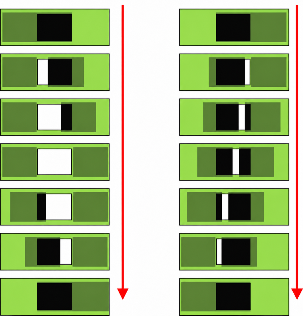
Symmetry

The mechanics rely on two carbon fiber or sandwich-type blades that move on a pair of linear ball bearings and are driven by two stepper motors and toothed belts. Steiner Shutters are highly symmetrical, and unlike most other shutter types, they don’t have a preferred direction of movement. Consequently, for consecutive exposures, the shutter blades move first from left to right and then from right to left. The control electronics hardware design is also symmetric. It consists of two identical microcontroller systems – one for each shutter blade.

Low Acceleration

A camera shutter has to guarantee precise exposure times. Moreover, exposure times must be the same at each point in the focal plane; exposures must be homogeneous. Most shutters (iris type, sector disk, slit type) try to achieve these goals by high-speed operation, at least if short exposure times are required. High speed implies high acceleration and deceleration. The corresponding energy has to be absorbed by the device – for spring-actuated types, usually within a very short (msec) braking period. Therefore, the shutter device’s lifetime and the vibrations shutter operation induces in the whole instrument are usually major issues.

The Steiner Shutters are impact-free, low-acceleration (i.e., low-power) devices. Their lifetime is less critical. For example, the shutter’s acceleration and deceleration during opening (7 m/s^2) are about an order of magnitude below the radially outward acceleration of a typical 60-100 mm iris-type shutter (opening time about 30 ms), not to mention the latter’s impact-like deceleration.

Precision Control

Instead of driving the shutter blades at high speed/acceleration, the 1 ms timing accuracy is achieved by a simple yet very precise motion control of both blades: The generation of every single stepper motor micro-step (25 µm per step) follows exactly a timetable which is derived from a given velocity profile and stored in µC RAM. Both blades are driven with identical timetables (i.e., velocity profiles), a prerequisite for homogeneous exposures. The trapezoidal velocity profile is programmable in software.

 The Mechanical Unit

Shutters are developed in various sizes, for single CCD cameras as well as for the largest mosaic cameras. A 60 mm square aperture shutter complete with control electronics and power supply is shown below.

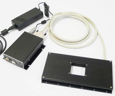
Despite the wide range of aperture sizes, the mechanics are essentially the same across all types. Everything is mounted on a single aluminum base plate with the aperture in the center. The shutter blades are usually made of carbon fiber. For the large PS1 shutter (e.g. Pan-STARRS, 480mm square aperture) a sandwich structure was used to reduce weight. Both blades move on linear ball bearings. The movement is monitored by encoders, and an absolute position reference is provided.

Endurance test

To prove the reliability of the moving parts, a complete drive section of a 200mm aperture) was copied, and an endurance test was performed.

Horizontal and vertical operation were possible. Most of the time, the setup was in the vertical position (up-down movement) with maximum load for the motor and toothed belt. Temperatures were: room, dome (6C), fridge (-20C). An operation (amplitude 220 mm) was initiated every second.

After 10 million cycles without failure (about 4 months of continuous operation), the experiment was switched off. No signs of critical abrasion were found. (After several years, this endurance test stand is still in use for motor tests.)

 Shutter Control Unit

The ShutterCU provides high-precision control of the shutter blade movement. Software command and hardware signal interfaces exist to connect the system to the camera and/or instrument control H/W and S/W.

Interfaces

The Interface to the camera/instrument control system is based on hardware control lines. Software command communication is also possible (ASCII over RS232, see below).

Hardware control lines

Three lines exist: (i) for shutter open/close operation, (ii) to indicate the “shutter closed” status, and (iii) for any error condition. These lines are accessible through the SubD9 connector labeled “Control”. Use of the status and error control lines is optional.

Serial command line (use is optional)

Through the RS232 line (SubD9 connector labelled “RS232”) a host can take control to get status information, to recover from error conditions and to redefine velocity profile parameters. Commands consist of 2 ASCII characters and up to 3 parameters (e.g. “ex 1000” for a 1000msec exposure).

The exposure start signal (falling edge) is continuously polled by software. The polling loop takes about 25µsec. This time delay sets the ultimate limit for the shortest possible exposure. In addition, the shortest possible exposure pulse is limited electronically to 300µsec.

Exposure control

The shutter can be operated in various ways:

• Manually: Press/release the open button to open/close the shutter.
• TTL compatible signal: Falling edge opens, rising edge closes the shutter. Input is via the connector labeled “Control”.
• By command: Send the “ex” command over the RS232 serial line to initiate a shutter operation (exposure time in msec). This is intended for testing and demonstration.

 The Firmware

All shutter operations are performed by the microcontroller firmware.

Initialization

After power-on or shutter reset (Reset button), the blades are moved for position calibration. Then the firmware starts polling the “shutter open/close” signal.

Blade movement

Shutter blade movements during opening or closing follow a trapezoidal velocity profile that is identical for both blades and both movement directions. It is characterized by 3 parameters: Acceleration, maximum velocity, and blade travel distance.

ShCU commands

For diagnostics, monitoring, or parameter modification, several commands allow communication with the ShCU via the RS232 connection. All commands consist of two lowercase command characters and numerical parameters separated by blank spaces. Each command sends its answer value (if defined) plus the prompt “c>”.

For illustration, a command sequence is shown which we recommend applying after unpacking a new shutter to familiarize yourself with the device and its control.

 Shutter Performance

Information given on this page is based on tests made with the 370 mm x 292 mm aperture OmegaCAM shutter and the 480 mm x 480 mm aperture PS1 shutter for the Pan-STARRS prototype telescope.

Shortest and longest exposure time

Because the opening and closing shutter blades can be moved independently, the shortest exposure time is essentially limited by the system’s response time to the shutter open/close signals. This depends first of all on the turnaround time of the firmware polling loop, which detects these signals (40 µsec). But in practice exposure times below 1 ms don’t make sense, as the non-homogeneities are typically of the order 300 – 500µsec. Therefore, the shortest possible exposure pulse is electronically limited to 300 µsec.

Exposure duration accuracy

The exposure duration accuracy has two aspects which are considered independently:

• The average exposure duration. Accuracy depends on how fast and how reproducibly the shutter reacts to the open/close signals. With a measured delay between exposure control signals and the first stepper motor step of 38 to 40 µs (the above-mentioned polling loop delay), this reaction time is far below the usually required upper limit of 10ms (or 1% at 1 s exposure time).
• The exposure homogeneity over the shutter aperture for a single exposure. This is discussed in what follows.

Non-uniform exposures occur if the movements of both shutter blades are not exactly identical. Limitations mainly come from stepper-motor resolution and mechanical tolerances, since the velocity profiles for both blades and both movement directions are the same within 1 µsec and independent of exposure time. Irregularities in the blade movement will therefore add/subtract a certain amount of time at the position in the aperture where they occur. Their effect on exposures then increases linearly with decreasing exposure time (and they are best detected at very short exposure times).

Based on these considerations, the exposure homogeneity was measured by adopting a procedure commonly used at telescopes: Flat field exposures taken with the exposure time in question are compared with exposures with significantly longer (50 x) exposure times, which serve as reference. Since no huge camera and no adequate optical setup were affordable to get real flat fields, the setup was slightly modified.

A homogeneity test stand was designed which allows us to take direct images of the shutter aperture. One important difference between this setup and the telescope configuration is that we get sharp images of the aperture plane. In contrast, each pixel in the telescope focal plane receives light through a cone whose diameter at the shutter position depends on the effective aperture ratio and the distance from the focal plane. The real telescope smooths out corresponding small-scale effects, while our setup images them well. This makes our setup more sensitive to non-homogeneities.

Testing equipment

A test stand was designed such that the shutter could be operated in vertical orientation. In terms of homogeneity, the vertical orientation is the most demanding: while the blades move up and down, the motors carry maximum load, and the difference between upward and downward motion is greatest. The test stand allows us to take images of the shutter aperture plane with a cryogenic CCD camera. The aperture is illuminated by a lightbox.

Data handling

We took several short-exposure images and coadded them to improve S/N. After subtracting the bias level, long and corresponding short exposures were divided by each other, and the result was normalized to an average of 1. All columns across the aperture (running parallel to the shutter blade movement direction) were averaged to further improve S/N. The resulting scans are shown below.

Searching for non-homogeneities at 0.2sec exposure time

We chose an exposure time of 0.2sec to demonstrate exposure homogeneity and quantify its limits. Reference exposures were 10sec long (i.e., a factor of 50).

We measured OmegaCAM shutter exposure homogeneity at 0.2 sec exposure time at two temperatures. A number of short exposures were coadded to improve S/N (left: 32, right:64). The abscissa covers the complete width of the shutter aperture (370mm). The diagrams show that the nonhomogeneities are well within +-0.3%. Residual curvatures in the scans are well explained by a shadowing effect that occurs only in our setup and will not exist on the real instrument.

By adding up a large number of short exposures, only systematic non-homogeneities can be detected. Randomly occurring effects are smoothed out. They will be discussed below.

Back-and-forth symmetry test

The shutter operates in either direction. The results presented so far show the average effect of both movements. Differences between the two directions are not expected since the shutter design is highly symmetric. However, all tests presented here were conducted with the shutter in the vertical position, with maximum load difference for opposite movement directions. If this has led to differences, they should be easily made visible by direct comparison. To do this, frames were separated according to the upward/downward direction, and homogeneity diagrams were calculated using frames taken with one movement direction as reference for those taken with the opposite direction.

Ratio of flats taken with opposite shutter blade motions at 0.2sec exposure time and two temperatures.

Randomly occurring inhomogeneities

By ratioing images averaged over many exposures, one can in principle only detect systematic inhomogeneities, but not random ones. No systematic search for random exposure inhomogeneities has been conducted over a large number of exposure operations. But there is little reason to suspect that random inhomogeneities would occur at a level that exceeds the systematic ones significantly – keeping in mind the shutter design and its principle of operation:

• oscillator-based stepper motor frequencies
• direct transmission of stepper motor rotation to blade translation through toothed belts.
• independent encoders.

The most probable source of significant random deviations of the blade motion from the velocity profile would be missing stepper motor steps (e.g. due to obstacles or exceedingly high friction). We check this after each blade movement by reading the corresponding encoder value. Deviations corresponding to timing errors of > 0.4 msec would trigger an error signal.

A very simple acoustic homogeneity test.

Non-homogeneities result from timing irregularities in the blade motions. At very short exposure times (a few msec), when the blades form a narrow slit, non-homogeneities of the same order would lead to collisions between the two blades. These collisions should be visible and audible. But even at exposure times of 1 msec, collisions were not detected (heard).